Pygrackle: Running Grackle in Python

Grackle comes with a Python interface, called Pygrackle, which provides access to all of Grackle’s functionality. Pygrackle requires the following Python packages:

• Cython

• flake8 (only required for the test suite)

• h5py

• matplotlib

• NumPy

• packaging (only required for the test suite)

• py.test (only required for the test suite)

• yt

The easiest thing to do is follow the instructions for installing yt, which will provide you with Cython, matplotlib, and NumPy. Flake8 and py.test can then be installed via pip.

You also need to have a fortran compiler installed (for building the Grackle library itself).

Installing Pygrackle

Currently, the only way to get Pygrackle is to build it from source.

There are 3 ways to build Pygrackle:

1. As a standalone, self-contained module. The build command creates a fresh build of the Grackle library and packages it with the Pygrackle module. (This is the recommended approach)

2. As a module that links to an external copy of Grackle that was compiled with the Classic build system. (This is consistent with the legacy approach for building Pygrackle).

3. As a module that links to an external copy of Grackle that was created with the CMake build system.

Currently, Pygrackle should be used with Grackle builds where OpenMP is disabled.

Warning

We strongly encourage you to use the first approach so that your Pygrackle installation is independent of other Grackle installations on your machine.

The latter 2 approaches are primarily intended for testing-purposes. If you use the latter 2 approaches, it’s your responsibility to ensure that you delete the old version of Pygrackle and reinstall it whenever the external Grackle library is updated. If you forget, Pygrackle may still work, but it’s more likely to produce a segmentation fault or (even worse!) silently give incorrect results.

1. Build Pygrackle as a standalone module (recommended)

To install Pygrackle, you just need to invoke the following from the root directory.

~/grackle $ pip install -v .

You can configure the exact C and Fortran compilers that are used for this by manipulating the CC and FC environment variables. If you must pass extra compiler flags to all invocations of the C or Fortran compiler, you can use the CFLAGS or FFLAGS environment variable.

If you encounter any compilation problems, you can also link Pygrackle against a version of the Grackle library that you already built.

(In the event that you are writing an external python package that depends on directly linking to the underlying Grackle library, be aware that the underlying organization of files in the resulting package may change)

2. Link to external Grackle library (built with Classic build system)

Prerequisite: This scenario assumes that you have already built Grackle with the Class build system.

To build Pygrackle, we use the PYGRACKLE_LEGACY_LINK environment variable to indicate that we want to that external build. Specifically, that variable must be configured as PYGRACKLE_LEGACY_LINK=classic.

~/grackle $ PYGRACKLE_LEGACY_LINK=classic pip install .

Note

We explicitly try to maintain the legacy behavior of the older setuptools-based python build-system. This means that we use the copy of the Grackle shared library from the build directory during linking (i.e. Pygrackle will happily build even if Grackle isn’t fully installed).

We then ASSUME that a copy of the Grackle shared library will be in a location known to the system, when you try to run Pygrackle. This could be a standard system location for libraries (on some systems you may need to invoke ldconfig after installation). This could also be a location specified by the relevant variable; LD_LIBRARY_PATH if you’re on Linux (or most unix-like systems) or DYLD_LIBRARY_PATH (if you’re on macOS)

3. Link to external Grackle library (built with the CMake build system)

Prerequisite: This scenario assumes that you have already built (and possibly installed) Grackle with the CMake build system. Specifically, that cmake build must have compiled Grackle as a shared library (the primary way to ensure this happens is by passing the -DBUILD_SHARED_LIBS=ON flag when using cmake to configure the build).

To build Pygrackle in this way, you must initialize either the Grackle_DIR environment variable or the Grackle_ROOT environment variable with the relevant path for your prebuilt Grackle library. This path can either point to cmake build directory (where Grackle is built) OR an installation directory.

We illustrates how to install Pygrackle under this approach down below. For the sake of example, we assume that we previously used cmake to build (and compile) Grackle as a shared library in a build directory called ~/grackle/build.

Default Case (libgrackle won’t move after building)Legacy Linking

The default command to build Pygrackle against a CMake-built is shown below. By default, this approach assumes that the Grackle shared library will never move. This means that issues will occur if you delete or move the Grackle library. (This is a necessary assumption in order to support build directories).

~/grackle $ Grackle_DIR=${PWD}/build pip install .

Testing Your Installation

To make sure everything is installed properly, you can try invoking pygrackle from the command line:

$ python -c "import pygrackle"

If this command executes without raising any errors, then you have successfully installed Pygrackle.

Installing Pygrackle Development Requirements

There are a handful of additional packages required for developing Grackle. For example, these will enable Testing and building the documentation locally. To install the development dependencies, repeat the last line of the pygrackle installation instructions with [dev] appended.

~/grackle $ pip install -e .[dev]

If you use zsh as your shell, you will need quotes around ‘.[dev]’.

~/grackle $ pip install -e '.[dev]'

Running the Example Scripts

A number of example scripts are available in the src/python/examples directory. These scripts provide examples of ways that Grackle can be used in simplified models, such as solving the temperature evolution of a parcel of gas at constant density or in a free-fall model. Each example will produce a figure as well as a dataset that can be loaded and analyzed with yt.

Editable Install Requirement

All of the example scripts discussed below use the following line to make a guess at where the Grackle input files are located.

Caution

This snippet is NOT part of the public API. It is a short-term solution that is being used until functionality proposed by GitHub PR #237 can be reviewed.

from pygrackle.utilities.data_path import grackle_data_dir

This currently ONLY works for an ‘editable’ Pygrackle installation (i.e., one installed with pip install -e . as directed above). In this case, it will be assumed that the data files can be found in a directory called input in the top level of the source repository.

Note

GitHub PR #235 is a pending pull request that seeks to add functionality to make this work in a regular Pygrackle installation (i.e. a non-‘editable’ install).

Cooling Rate Figure Example

This sets up a one-dimensional grid at a constant density with logarithmically spaced temperatures from 10 K to 10⁹ K. Radiative cooling is disabled and the chemistry solver is iterated until the species fractions have converged. The cooling time is then calculated and used to compute the cooling rate.

~/grackle/src/python/examples $ python cooling_rate.py

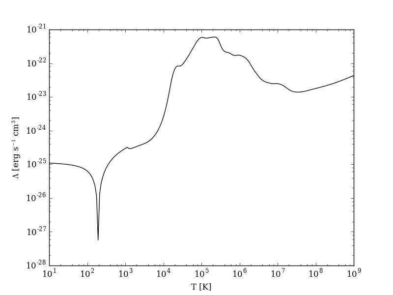
After the script runs, and hdf5 file will be created with a similar name. This can be loaded in with yt.

>>> import yt
>>> ds = yt.load("cooling_rate.h5")
>>> print ds.data["temperature"]
[  1.00000000e+01   1.09698580e+01   1.20337784e+01   1.32008840e+01, ...,
   7.57525026e+08   8.30994195e+08   9.11588830e+08   1.00000000e+09] K
>>> print ds.data["cooling_rate"]
[  1.09233398e-25   1.08692516e-25   1.08117583e-25   1.07505345e-25, ...,
   3.77902570e-23   3.94523273e-23   4.12003667e-23   4.30376998e-23] cm**3*erg/s

Cooling Cell Example

This sets up a single grid cell with an initial density and temperature and solves the chemistry and cooling for a given amount of time. The resulting dataset gives the values of the densities, temperatures, and mean molecular weights for all times.

~/grackle/src/python/examples $ python cooling_cell.py

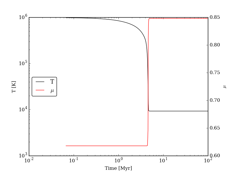
>>> import yt
>>> ds = yt.load("cooling_cell.h5")
>>> print ds.data["time"].to("Myr")
YTArray([  0.00000000e+00,   6.74660169e-02,   1.34932034e-01, ...,
         9.98497051e+01,   9.99171711e+01,   9.99846371e+01]) Myr
>>> print ds.data["temperature"]
YTArray([ 990014.56406726,  980007.32720091,  969992.99066987, ...,
          9263.81515866,    9263.81515824,    9263.81515865]) K

Free-Fall Collapse Example

This sets up a single grid cell with an initial number density of 1 cm^-3. The density increases with time following a free-fall collapse model. As the density increases, thermal energy is added to model heating via adiabatic compression. This can be useful for testing chemistry networks over a large range in density.

~/grackle/src/python/examples $ python freefall.py

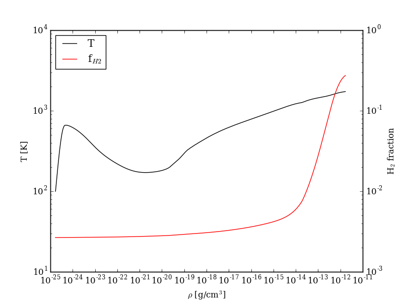
The resulting dataset can be analyzed similarly as above.

>>> import yt
>>> ds = yt.load("freefall.h5")
>>> print ds.data["time"].to("Myr")
[   0.            0.45900816    0.91572127 ...,  219.90360841  219.90360855
  219.9036087 ] Myr
>>> print ds.data["density"]
[  1.67373522e-25   1.69059895e-25   1.70763258e-25 ...,   1.65068531e-12
   1.66121253e-12   1.67178981e-12] g/cm**3
>>> print ds.data["temperature"]
[   99.94958248   100.61345564   101.28160228 ...,  1728.89321898
  1729.32604568  1729.75744287] K

Using Grackle with yt

This example illustrates how Grackle functionality can be called using simulation datasets loaded with yt as input. Note, below we invoke Python with the -i flag to keep the interpreter running. The second block is assumed to happen within the same session.

~/grackle/src/python/examples $ python -i yt_grackle.py

>>> print (sp['gas', 'grackle_cooling_time'].to('Myr'))
[-5.33399975 -5.68132287 -6.04043746 ... -0.44279721 -0.37466095
 -0.19981158] Myr
>>> print (sp['gas', 'grackle_temperature'])
[12937.90890302 12953.99126155 13234.96820101 ... 11824.51319307
 11588.16161462 10173.0168747 ] K

Through pygrackle, the following yt fields are defined:

• ('gas', 'grackle_cooling_time')

• ('gas', 'grackle_gamma')

• ('gas', 'grackle_molecular_weight')

• ('gas', 'grackle_pressure')

• ('gas', 'grackle_temperature')

• ('gas', 'grackle_dust_temperature')

These fields are created after calling the add_grackle_fields function. This function will initialize Grackle with settings from parameters in the loaded dataset. Optionally, parameters can be specified manually to override.